12.3 Example of Interpolator usage
12.4 Using a cubic-spline interpolator
The Interpolator class defines the functionality for an important and powerful set of behaviors that deserve extra mention. The behaviors derived from Interpolator allow an objects current state to be interpolated between a set of defined states as a function of time.
This chapter introduces the Interpolator classes and the Alpha class, which is used to control the speed of interpolation.
java.lang.Object
  |
  +--javax.media.j3d.SceneGraphObject
        |
        +--javax.media.j3d.Node
              |
              +--javax.media.j3d.Leaf
                    |
                    +--javax.media.j3d.Behavior
                          |
                          +--javax.media.j3d.Interpolator
Java 3D includes a rich set of behaviors for interpolating an object between states. These behaviors are important for many animation and visualization applications and are covered in detail in this section. Interpolator behaviors can be used to interpolate an objects:
Switch valueToggle Switch Nodes visible child based on time
All the Interpolation classes require an Alpha object. The Alpha class is used to convert the current time to a value between 0 and 1this value is then used by the Interpolator to perform its specific action. The Alpha class is described in section 12.2.
java.lang.Object
  |
  +--javax.media.j3d.Alpha
A good understanding of the Alpha class is key to using all the Interpolator behaviors. The Alpha class defines a function that converts the current time (in milliseconds) to a value between 0 and 1 (alpha value). The alpha value can then be used by the Interpolator to produce the desired interpolation between specified end states.
For example, a PositionInterpolator might be used to move an object between position (0,0,0) and (0,0,5) in 10 seconds. To achieve the desired result, an Alpha object must be created that returns 0 at 0 seconds and 1 at 10 seconds. The PositionInterpolator can then use the Alpha object to create the desired z coordinate (table 12.1).
| Time (seconds) | Alpha | Z Coordinate |
|---|---|---|
| 0 | 0 | 0 * 5 = 0 |
| 5 | 0.5 | 0.5 * 5 = 2.5 |
| 10 | 1 | 1 * 5 = 5 |
The Alpha class uses a parameterized function to convert time values to alpha values between 0 and 1.
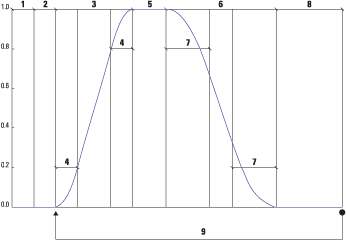
Figure 12.1 illustrates the basic shape of the functions that can be created using the Alpha class. Nine parameters can be used to create a customized Alpha function are listed there.

Alpha class: triggerTime (1), phase delay (2), increasing alpha (3), increasing alpha ramp (4), at one (5), decreasing alpha (6), decreasing alpha ramp (7), at zero (8), and loopCount (9)
The increasing alpha phase (3) is composed of three potential sections, as is the decreasing alpha phase (6). The values of increasing alpha ramp (4) and decreasing alpha ramp (7) define symmetrical acceleration and deceleration of the Alpha value at the beginning and end of the phase. These quadratic sections help to smooth the transition from 0 to 1 (increasing alpha) or 1 to 0 (decreasing alpha). Note that the Alpha value varies linearly between the quadratic sections. The loopCount parameter (9) allows Alpha functions to be repeated (a fixed number of times or infinitely) by joining Alpha functions end to end.
Run the AlphaTest example and interactively modify the nine parameters to get a good feel for how to parameterize an Alpha object for your application (figure 12.2).
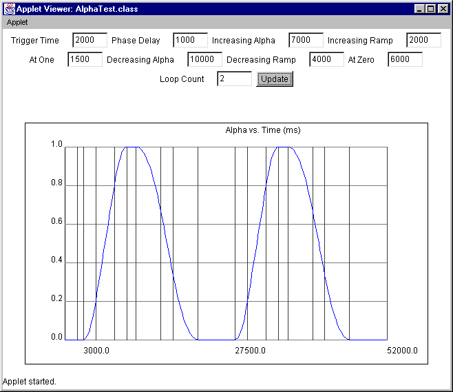
Alpha object to be parameterized interactively and plots the resulting Alpha function
| NOTE |
While testing the AlphaTest example, I ran into an interesting bug in the Alpha class. If either the increasing alpha ramp or decreasing alpha ramp parameter is set to zero, the other will also be set to zero. You can work around this bug by setting the parameter to 1 millisecond instead of 0 milliseconds. |
You can, of course, derive your own class from Alpha to implement your own Alpha function. The FileAlpha class from the CustomAlphaTest examples loads times and alpha values from a text file and linearly interpolates between them.
| From the file Values.xls from the CustomAlphaTest example |
0     0
1000  0.1
3000  0.4
4000  0.2
6000  0.8
10000 0.5
12000 0.1
14000 1.0
16000 0.1![]()
The text file defines an ordered series of time and alpha value pairs (figure 12.3). Times are specified in milliseconds.
The FileAlpha class overrides the following Alpha methods.
public void setStartTime(long l)
public long getStartTime()
public void setLoopCount( int i )
public int getLoopCount()
public boolean finished()
public float value( long time )
Please refer to the FileAlpha class for details.
The CustomAlphaTest is also interesting in that it interpolates the position of a ColorCube using the FileAlpha and plots the value and time of the FileAlpha on the graph shown in figure 12.3.
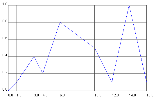
FileAlpha class loads times and Alpha values from a file and linearly interpolates between them to provide a highly flexible Alpha function
An Alpha class is very simpleit converts a time value in milliseconds to a value between 0 and 1. The built-in Alpha class defines all the parameters for an Alpha function to implement a common class of onset, peak, offset activation functions.
A custom Alpha function, such as FileAlpha, is a very powerful mechanism to feed application-specific data into one of the Interpolator-derived classes. An application might define an Alpha class that samples data straight from a communications port, or reads precomputed data from a file. The output from the custom Alpha class can then be used to parameterize a wide variety of Interpolators.
Alpha classes are used in conjunction with Interpolators, but they do not do anything visible themselves. Their prime purpose in Java 3D is to provide input to the Interpolator classes. Interpolators are the subjects of section 12.3, so read on.
java.lang.Object
  |
  +--javax.media.j3d.SceneGraphObject
        |
        +--javax.media.j3d.Node
              |
              +--javax.media.j3d.Leaf
                    |
                    +--javax.media.j3d.Behavior
                          |
                          +--javax.media.j3d.Interpolator
The Java 3D Interpolators were explored using the InterpolatorTest and the SplineInterpolatorTest examples. The InterpolatorTest example demonstrates using the following Interpolators:
The SwitchValueInterpolator is used to cycle through the children of a Switch Node based on the output from an Alpha object. The SwitchValueInterpolator maps the output from the Alpha into a current visible child Node using the following algorithm:
float f = alpha.value();
int i = firstSwitchIndex +
  (int)(f * (float)(childCount - 1) + 0.5F);
target.setWhichChild(i);
Note that the Switch Node passed to the SwitchInterpolator must have the Switch.ALLOW_SWITCH_WRITE capability.
//create the Switch Node
Switch switchNode = new Switch();
//set the WRITE capability
switchNode.setCapability( Switch.ALLOW_SWITCH_WRITE );
//add children to switchNode here
//create the Alpha for the Interpolator
Alpha alpha = new Alpha( -1,
Alpha.INCREASING_ENABLE | Alpha.DECREASING_ENABLE,
500,
100,
5000,
2000,
1000,
5000,
2000,
500 );
//create the SwitchInterpolator and pass the Alpha
//and a Switch Node
Interpolator switchInterpolator =
new SwitchValueInterpolator( alpha, switchNode );
//add the Interpolator to a parent BranchGroup
//and set Scheduling Bounds
BranchGroup bg = new BranchGroup();
bg.addChild( interpolator );
interpolator.setSchedulingBounds( getApplicationBounds() );The ColorInterpolator can be used to linearly interpolate the Material diffuse color of an Appearance between two extremes. Note that the Material must have the ALLOW_COMPONENT_WRITE capability bit set.
//create an Appearance
Appearance app = new Appearance();
//create a Material and assign an initial color
Color3f objColor = new Color3f(1.0f, 0.7f, 0.8f);
Color3f black = new Color3f(0.0f, 0.0f, 0.0f);
Material mat =
new Material(objColor, black, objColor, black, 80.0f);
//ensure the Interpolator has WRITE access to the Material
mat.setCapability( Material.ALLOW_COMPONENT_WRITE );
//assign the Material to the Appearance
app.setMaterial( mat );
//create the Interpolatorby default interpolate
//between black and white
Interpolator interpolator =
new ColorInterpolator( alpha, app.getMaterial() );The PositionInterpolator can be used to linearly interpolate between two x, y, z positions. The PositionInterpolator modifies a TransformGroup, which will in turn affect the position of all its child Nodes. The TransformGroup must have the ALLOW_TRANSFORM_WRITE capability set.
//create the TransformGroup
TransformGroup tg = new TransformGroup();
tg.setCapability(TransformGroup.ALLOW_TRANSFORM_WRITE);
tg.setCapability(TransformGroup.ALLOW_TRANSFORM_READ);
//create the Interpolatorby default interpolate
//between x = 0 and x = 1
Interpolator interpolator = new PositionInterpolator ( alpha, tg );The RotationInterpolator can be used to linearly interpolate between two sets of axis angle rotations. The RotationInterpolator modifies a TransformGroup, which will in turn affect the position of all its child Nodes. The TransformGroup must have the ALLOW_TRANSFORM_WRITE capability set.
//create the Interpolatorby default interpolate
//between Y angle = 0 and Y angle = 2p
Interpolator interpolator = new RotationInterpolator ( alpha, tg );The ScaleInterpolator can be used to linearly interpolate between two scale values for an axis. The ScaleInterpolator modifies a TransformGroup, which will in turn affect the position of all its child Nodes. The TransformGroup must have the ALLOW_TRANSFORM_WRITE capability set.
//create the Interpolatorby default interpolate
//between a uniform scale of 0 and 1
Interpolator interpolator = new ScaleInterpolator ( alpha, tg );The TransparencyInterpolator can be used to linearly interpolate between two transparency values. The TransparencyInterpolator modifies an Appearances TransparencyAttributes. The TransparencyAttributes must have the ALLOW_VALUE_WRITE capability set.
//create the TransparencyAttributes
TransparencyAttributes transparency = new TransparencyAttributes();

//set the required capability bit
transparency.setCapability(
  TransparencyAttributes.ALLOW_VALUE_WRITE );

//set the transparency mode
transparency.setTransparencyMode( TransparencyAttributes.NICEST );

//assign the transparency to an Appearance
app.setTransparencyAttributes( transparency );

//create the interpolator and interpolate
//between 0 (opaque) and 0.8.
Interpolator interpolator = new TransparencyInterpolator( alpha, app.getTransparencyAttributes(), 0, 0.8f );The RotPosScalePathInterpolator is the most flexible of all the PathInterpolators. As its name suggests, it allows the rotation, position, and scale of a TransformGroup to be modified.
Rotations, positions, and scales are specified at a series of Alpha values (or knots). The rotation, position, and scale defines a pose that, along with the time information, allows the Interpolator to linearly interpolate between poses based on the Alpha value and the defined knots.
As the name knots implies, a useful way to visualize the interpolator is as a string stretched taut between a number of points. Each point is called a knot, and as well as having an Alpha value (time) when the interpolator is to reach the knot it also possesses position, scale, and rotation information (a pose). The distance between knots defines the speed at which the interpolation between values must occur.
Knots are specified using float values between 0 and 1, where 0 is the knot used at Alpha value 0 and 1 is the knot used at Alpha time 1. The array of knot values defines a mapping from Alpha value to pose information. The knot values must increase from 0 to 1 in the knot array.
//define the knots array that map from Alpha to pose index
float[] knots = {0.0f, 0.1f, 0.2f, 0.3f, 0.4f,
                 0.6f, 0.8f, 0.9f, 1.0f};

//create array with 9 poses: containing rotation, position
//and scale values
Quat4f[] quats = new Quat4f[9];
Point3f[] positions = new Point3f[9];
float[] scales = {0.2f, 0.5f, 0.8f, 2.3f, 5.4f,
                  0.6f, 0.4f, 0.2f, 0.1f};

//define the rotation values for each of the 9 poses
quats[0] = new Quat4f(0.3f, 1.0f, 1.0f, 0.0f);
quats[1] = new Quat4f(1.0f, 0.0f, 0.0f, 0.3f);
quats[2] = new Quat4f(0.2f, 1.0f, 0.0f, 0.0f);
quats[3] = new Quat4f(0.0f, 0.2f, 1.0f, 0.0f);
quats[4] = new Quat4f(1.0f, 0.0f, 0.4f, 0.0f);
quats[5] = new Quat4f(0.0f, 1.0f, 1.0f, 0.2f);
quats[6] = new Quat4f(0.3f, 0.3f, 0.0f, 0.0f);
quats[7] = new Quat4f(1.0f, 0.0f, 1.0f, 1.0f);
quats[8] = quats[0];

//define the positions for each of the 9 poses
positions[0]= new Point3f(0.0f,  0.0f, -1.0f);
positions[1]= new Point3f(1.0f, -2.0f, -2.0f);
positions[2]= new Point3f(-2.0f,  2.0f, -3.0f);
positions[3]= new Point3f(1.0f,  1.0f, -4.0f);
positions[4]= new Point3f(-4.0f, -2.0f, -5.0f);
positions[5]= new Point3f(2.0f,  0.3f, -6.0f);
positions[6]= new Point3f(-4.0f,  0.5f, -7.0f);
positions[7]= new Point3f(0.0f, -1.5f, -4.0f);
positions[8]= positions[0];

//create the interpolator and pass Alpha, TransformGroup,
//knots, and pose information
RotPosScalePathInterpolator rotPosScalePathInterplator = new RotPosScalePathInterpolator(
 alpha,
 tg,
 new Transform3D(),
 knots,
 quats,
 positions,
 scales );
As you can see, the rotation angles are specified using the Quat4f class. The Quat4f class specifies a rotation as a quaternion. The following is a description of quaternions, taken from the excellent Matrix and Quaternion FAQ. The FAQ can be found online and it currently maintained by Andreas Junghanns at http://www.cs.ualberta.ca/~andreas/math/matrfaq_latest.html.
Quaternions extend the concept of rotation in three dimensions to rotation in four dimensions. This avoids the problem of gimbal-lock and allows for the implementation of smooth and continuous rotation. In effect, they may be considered to add an additional rotation angle to spherical coordinates: longitude, latitude, and rotation angles. A Quaternion is defined using four floating point values |x y z w|. These are calculated from the combination of the three coordinates of the rotation axis and the rotation angle.
Unfortunately most people do not think readily in quaternions, so the following two conversion functions are useful to help create quaternions from axis or Euler angles. The algorithms for the functions were taken from the Matrix and Quaternion FAQ. I encourage you to check the FAQ for updates, optimizations and corrections to this code.
| From InterpolatorTest.java |
//Quat4f createQuaternionFromAxisAndAngle
//( Vector3d axis, double angle )
{
 double sin_a = Math.sin( angle / 2 );
 double cos_a = Math.cos( angle / 2 );

 //use a vector so we can call normalize
 Vector4f q = new Vector4f();

 q.x = (float) (axis.x * sin_a);
 q.y = (float) (axis.y * sin_a);
 q.z = (float) (axis.z * sin_a);
 q.w = (float) cos_a;

 //It is best to normalize the quaternion
 //so that only rotation information is used
 q.normalize();

 //convert to a Quat4f and return
 return new Quat4f( q );
}

//Quat4f createQuaternionFromEuler( double angleX,
//double angleY, double angleZ )
{
 //simply call createQuaternionFromAxisAndAngle for each axis
 //and multiply the results
 Quat4f qx = createQuaternionFromAxisAndAngle(
    new Vector3d(1,0,0), angleX );
 Quat4f qy = createQuaternionFromAxisAndAngle(
    new Vector3d(0,1,0), angleY );
 Quat4f qz = createQuaternionFromAxisAndAngle(
    new Vector3d(0,0,1), angleZ );

 //qx = qx * qy
 qx.mul( qy );

 //qx = qx * qz
 qx.mul( qz );

 return qx;
}![]()
The InterpolatorTest example creates a Switch Node and attaches a SwitchInterpolator. A custom Alpha class (RandomAlpha) is used to generate Alpha values for the SwitchInterpolator. The RandomAlpha generates a random Alpha value (between 0 and 1) every 10 seconds. This causes the SwitchInterpolator to randomly switch between child Nodes every 10 seconds.
The Switch Node has six child Nodes:
Group containing a ColorInterpolator: Operates on an Appearance.
Group containing a PositionInterpolator: Operates on a TransformGroup.
Group containing a RotationInterpolator: Operates on a TransformGroup.
Group containing a ScaleInterpolator: Operates on a TransformGroup.
Group containing a TransparencyInterpolator: Operates on an Appearance.
Group containing a RotPosScaleInterpolator: Operates on a TransformGroup.
Each Group also contains a Link Node to a common SharedGroup. The SharedGroup contains a TransformGroup with a child Shape3D. The parent TransformGroup is passed to each Interpolator that requires a TransformGroup, while the Shape3Ds Appearance is passed to each Interpolator that requires an Appearance. A Text2D is also created with the name of the Interpolator as text so that the current active Interpolator can be seen. See figure 12.4.
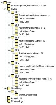
InterpolatorTest example
The InterpolatorTest example exploits a useful feature of Behaviors: when the Switch changes its active child Node, the Behaviors of the inactive child Nodes are no longer scheduled. In this way, the SwitchInterpolator that randomly selects child Nodes (using the RandomAlpha class) also activates a single Behaviorinactive Behaviors are no longer processed even though they are still enabled.
The RandomAlpha class is very simple:
//This class defines an Alpha class that returns
//a random value every N milliseconds.
public class RandomAlpha extends Alpha
{
 protected long      m_LastQueryTime = 0;
 protected float      m_Alpha = 0;
 protected final int    m_kUpdateInterval = 10000;

 public RandomAlpha()
 {
 }

//core method override returns the Alpha value for a given time
public float value( long time )
 {
  if( System.currentTimeMillis()
       - m_LastQueryTime > m_kUpdateInterval )
  {
   m_LastQueryTime = System.currentTimeMillis();
   m_Alpha = (float) Math.random();
  }

  return m_Alpha;
 }
}Java 3D includes a class to perform cubic-spline interpolation of position, rotation, and scale between key frames. The class uses the Kochanek-Bartels (K-B) algorithm to allow smooth interpolation between key frames (knots), which specify pose and interpolation information. Unlike linear interpolation, which suffers from potential discontinuities at control points (knots), K-B interpolation, while guaranteeing that the path passes through all the control points, varies the path smoothly. Instead of a piece of taut string strung between control points, the analogy is closer to a springy rod that passes through each point.
The K-B algorithm is fairly complex, and a discussion of the mathematics behind the algorithm is beyond the scope of this practical book. There are a number of very good online resources that describe the algorithm in detail. In addition, because the Interpolator class that implements the algorithm is in the Java 3D utils package, all the source code is available for inspection.
The good news is that the algorithm is extremely flexible and allows very fine control over the interpolated path. Each key frame, along with all the pose information (position, rotation, scale), also defines the following three parameters:
As with most terms in this book, a picture is worth a thousand words, so see figures 12.5, 12.6, and 12.7, which illustrate the K-B parameters.
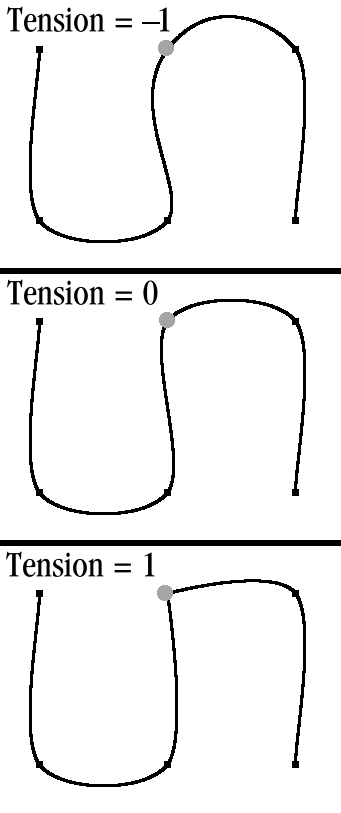
tension parameter at a key frame on a 2D K-B spline curve
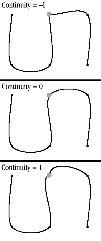
continuity parameter at a key frame on a 2D K-B spline curve
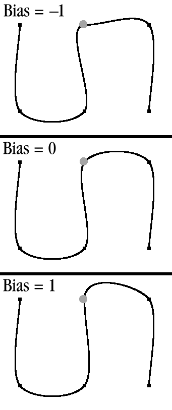
bias parameter at a key frame on a 2D K-B spline curve
The tension parameter controls the length of the curve segments either side of a key frame. The higher the tension, the shorter the segments.
The continuity parameter enables you to purposefully introduce discontinuities into the path. The path can either mimic a sharp corner at the key frame (1) or overshoot the key frame and slingshot back (1).
The bias parameter enables you to apportion tension at a key frame to each curve segment either side of the key frame. In this way the path is skewed about the key frame, with the segment on one side of the key frame slacker than the segment on the other side.
SplineInterpolatorTest is one of the most ambitious examples of the book. When I thought of animating an object using a spline curve, I thought of tracking a camera along a spline curve and rendering the results. My initial idea was to model an architectural or city fly-over, and the example grew from there.
SplineInterpolatorTest creates a virtual model of the city of Boston. The example loads a predefined spline curve from a file and takes the viewer on a virtual flight around the city (figures 12.8, 12.9, and 12.10).
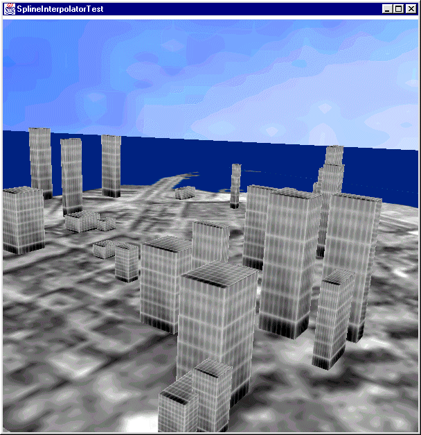
SplineInterpolatorTest example. Take a virtual fly-over of Boston city center
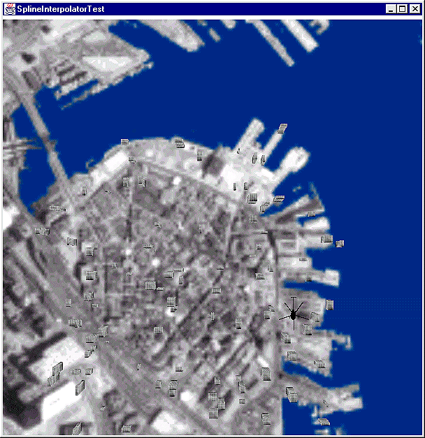
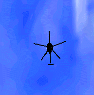
SplineInterpolatorTest dynamically switches to a low-resolution image of the whole of the city. One of the orbiting helicopters is visible in the frame
The virtual city is composed of the following elements:
Background Sphere.
Boxes).
PointSound source. The 3D sound engine generates 3D spatial sound from the three sound sources.
The rendered results are very pleasing, and the smoothness of the spline based animation gives a nice impression of movement and acceleration through the generated world. The satellite images were downloaded from the Microsoft Terraserver satellite image database. Terraserver is very useful in that different resolution images (i.e., from 32 meters per pixel down to 1 meter per pixel) can be easily downloaded. It allows a LOD behavior to be used, so that a high-resolution image appears when the viewer is close to the city and a lower resolution image appears when the viewer is far above the city. Both texture images are 256 × 256 pixels in size, and hence should be supported by hardware renderers.
To support the functionality required for the example, a base class was created for defining the behaviors, geometry, and appearance for the objects in the world. For an application of this complexity, the approach taken in most example code, which is to throw everything in the Applet class, was clearly not going to work. What was required was an OO design that empowered the objects within the world with the abilities they required. These abilities include:
Alpha object to animate the object.
These chores are handled by the ComplexObject class, which allows the main code of the application to deal with the objects themselves, and not with TransformGroups, sounds, appearances, and the like. This keeps the reusable functionality low in the class hierarchy and puts the application-specific details in super classes and the main Applet class itself.
The code for the example is obviously too long to be shown in full, so some interesting highlights will be discussed. The source code for ComplexObject is in the org.selman.java3d.book package.
//create a Switch group that contains two versions of the world:
//The first is a high resolution version, and the second is a
//lower resolution version.
public Group createLodLand( Group g )
{
 Switch switchNode = new Switch();
 switchNode.setCapability( Switch.ALLOW_SWITCH_WRITE );

 Group hiResGroup = createLand( switchNode );
 createEnvirons( switchNode );

//Create a DistanceLOD that will select the child
//of the Switch node based on distance. Here we are
//selecting child 0 (high res) if we are closer
//than 180 units to 0,0,0, and child 1 (low res) otherwise.
 float[] distanceArray = {180};

 DistanceLOD distanceLod = new DistanceLOD( distanceArray );
 distanceLod.setSchedulingBounds( getApplicationBounds() );
 distanceLod.addSwitch( switchNode );

 g.addChild( distanceLod );
 g.addChild( switchNode );

 return hiResGroup;
}The following code is used to read in a series of key frames from a disk file. Defining key frames by hand takes a lot of trial and error, so it is very desirable to be able to quickly modify the key frame file and rerun the application rather than having to recompile.
A utility method was written to read the data for a series of key frames from a disk file. The format of the file is as follows:
For example, the spline curve that the viewer is interpolated along is defined as follows, from rotate_viewer_spline.xls:
0.0
5 6 5
-0.4 0 0
1 1 1
0 1 0
0

0.3
2 4 10
1.0  0.2 0
1 1 1
0 0 0
0

0.5
-2 4 8
-0.3 0.6 0.2
1 1 1
-1 1 -1
0

0.7
-2 5 10
-0.4 -0.6 0.5
1 1 1
-1 1 -1
0

0.8
-1 4 5
-0.6 -0.9 -0.2
1 1 1
1 1 1
0

0.9
0 10 15
-1.2 0 0
1 1 1
1 0 1
0

1.0
0 52 0
-1.5 0 0
1 1 1
0 1 1
0
The utility method to read and create the key frame array is simply the following:
| From Utils.java in the org.selman.java3d.book package |
static public TCBKeyFrame[] readKeyFrames( URL urlKeyframes )
{
 StringBuffer szBufferData = readFile( urlKeyframes );

 if( szBufferData == null )
  return null;

 Vector keyFramesVector = new Vector();

 //create a tokenizer to tokenize the input file at whitespace
 java.util.StringTokenizer tokenizer =
   new java.util.StringTokenizer( szBufferData.toString() );

 /*
  * Each keyframe is defined as follows:
  * - knot (0 >= k <= 1)
  * - position (x,y,z)
  * - rotation (rx,ry,rz)
  * - scale (x,y,z)
  * - tension (-1 >= t <= 1)
  * - continuity (-1 >= c <= 1)
  * - bias (-1 >= b <= 1)
  * - linear (int - 0 or 1)
  */
 while( true )
 {
  try
  {
   float knot = Float.parseFloat( tokenizer.nextToken() );

   float posX = Float.parseFloat( tokenizer.nextToken() );
   float posY = Float.parseFloat( tokenizer.nextToken() );
   float posZ = Float.parseFloat( tokenizer.nextToken() );

   float rotX = Float.parseFloat( tokenizer.nextToken() );
   float rotY = Float.parseFloat( tokenizer.nextToken() );
   float rotZ = Float.parseFloat( tokenizer.nextToken() );

   float scaleX = Float.parseFloat( tokenizer.nextToken() );
   float scaleY = Float.parseFloat( tokenizer.nextToken() );
   float scaleZ = Float.parseFloat( tokenizer.nextToken() );

   float tension = Float.parseFloat( tokenizer.nextToken() );
   float continuity = Float.parseFloat( tokenizer.nextToken() );
   float bias = Float.parseFloat( tokenizer.nextToken() );

   int linear = Integer.parseInt( tokenizer.nextToken() );

   //create the actual keyframe from the data just read
   TCBKeyFrame keyframe = new TCBKeyFrame(
    knot,
    linear,
    new Point3f( posX, posY, posZ ),
    createQuaternionFromEuler( rotX, rotY, rotZ ),
    new Point3f( scaleX, scaleY, scaleZ ),
    tension,
    continuity,
    bias );

   keyFramesVector.add( keyframe );
  }
  catch( Exception e )
  {
   break;
  }
 }

 //create the return structure and populate
 TCBKeyFrame[] keysReturn =
   new TCBKeyFrame[ keyFramesVector.size() ];

 for( int n = 0; n < keysReturn.length; n++ )
  keysReturn[n] = (TCBKeyFrame) keyFramesVector.get( n );

 //return the array
 return keysReturn;
}![]()
To create the background for the example we create a Sphere, assign a texture image to the Sphere and then assign the Sphere to a Background node. Note that because the viewer of the scene is within the Sphere the normal vectors assigned to the vertices of the Sphere must be created with the Primitive.GENERATE_NORMALS_INWARD option.
| From SplineInterpolatorTest.java |
//we want a texture-mapped background of a sky
protected Background createBackground()
{
 //add the sky backdrop
 Background back = new Background();
 back.setApplicationBounds( getApplicationBounds() );

 BranchGroup bgGeometry = new BranchGroup();

 //create an appearance and assign the texture image
 Appearance app = new Appearance();
 Texture tex = new TextureLoader( "sky.gif", this).getTexture();
 app.setTexture( tex );

 Sphere sphere =
  new Sphere( 1.0f, Primitive.GENERATE_TEXTURE_COORDS |
                    Primitive.GENERATE_NORMALS_INWARD,
              app );

 bgGeometry.addChild( sphere );
 back.setGeometry( bgGeometry );

 return back;
}![]()
The distance over which the PointSounds created for the three helicopters can be heard is controlled by three factors: (1) the ViewPlatforms activation radius, (2) the scheduling bounds of the Sound, and (3) distance/gain parameters of the PointSound itself.
A PointSound is potentially audible when the ViewPlatforms activation radius intersects the scheduling bounds for the Sound. The actual volume of the mixed sound is controlled by the distance/gain parameters for the PointSound.
| From Helicopter.java |
//Return the scheduling bounds for the Helicopters sound
protected Bounds getSoundSchedulingBounds( boolean bCollide )
{
return new BoundingSphere( new Point3d(0,0,0), 20 );
}![]()
The getSoundDistanceGain method returns an array of Point2f objects that define how the volume of the sound attenuates with distance. In the following example the sound is at 20 percent of its maximum intensity at 2 units distance and at 5 percent of maximum intensity at 20 units distance.
protected Point2f[] getSoundDistanceGain( boolean bCollide )
{
 Point2f[] gainArray = new Point2f[2];

 gainArray[0] = new Point2f( 2, 0.2f );
 gainArray[1] = new Point2f( 20, 0.05f );

 return gainArray;
}This discussion of Interpolators and the SplineInterpolatorTest example should have alerted you to some of the power of the interpolator behaviors built into Java 3D. The support for such high-level features as interpolators in Java 3D is a real time saver. Just think about having to implement this functionality by hand.